> ## Documentation Index
> Fetch the complete documentation index at: https://docs.neuroencoder.com/llms.txt
> Use this file to discover all available pages before exploring further.

# Visualization

> Interactive Embedding Atlas

```python theme={null}
import neuroencoder as ne
ne.explore(embeddings)
```

Launches Apple's open-source [Embedding Atlas](https://github.com/apple/embedding-atlas) inline in Jupyter. Defaults: time coloring, side panels hidden — a clean canvas you can pan and zoom.

<Frame caption="EEGBCI motor imagery (PhysioNet, public). 5 subjects × 6 runs = 30 recordings, 2,216 epochs (sliding 30s windows at 1s stride), embedded with the MRL model. Color = recording time.">
  <img src="https://mintcdn.com/ethzurich-0a1ee124/ZfpYpuMxcfdV-ZM-/images/atlas-eegbci.png?fit=max&auto=format&n=ZfpYpuMxcfdV-ZM-&q=85&s=9fc0346b4ce497033a61ad7c341cba50" alt="Apple Embedding Atlas: EEGBCI motor imagery embeddings" width="3600" height="2200" data-path="images/atlas-eegbci.png" />
</Frame>

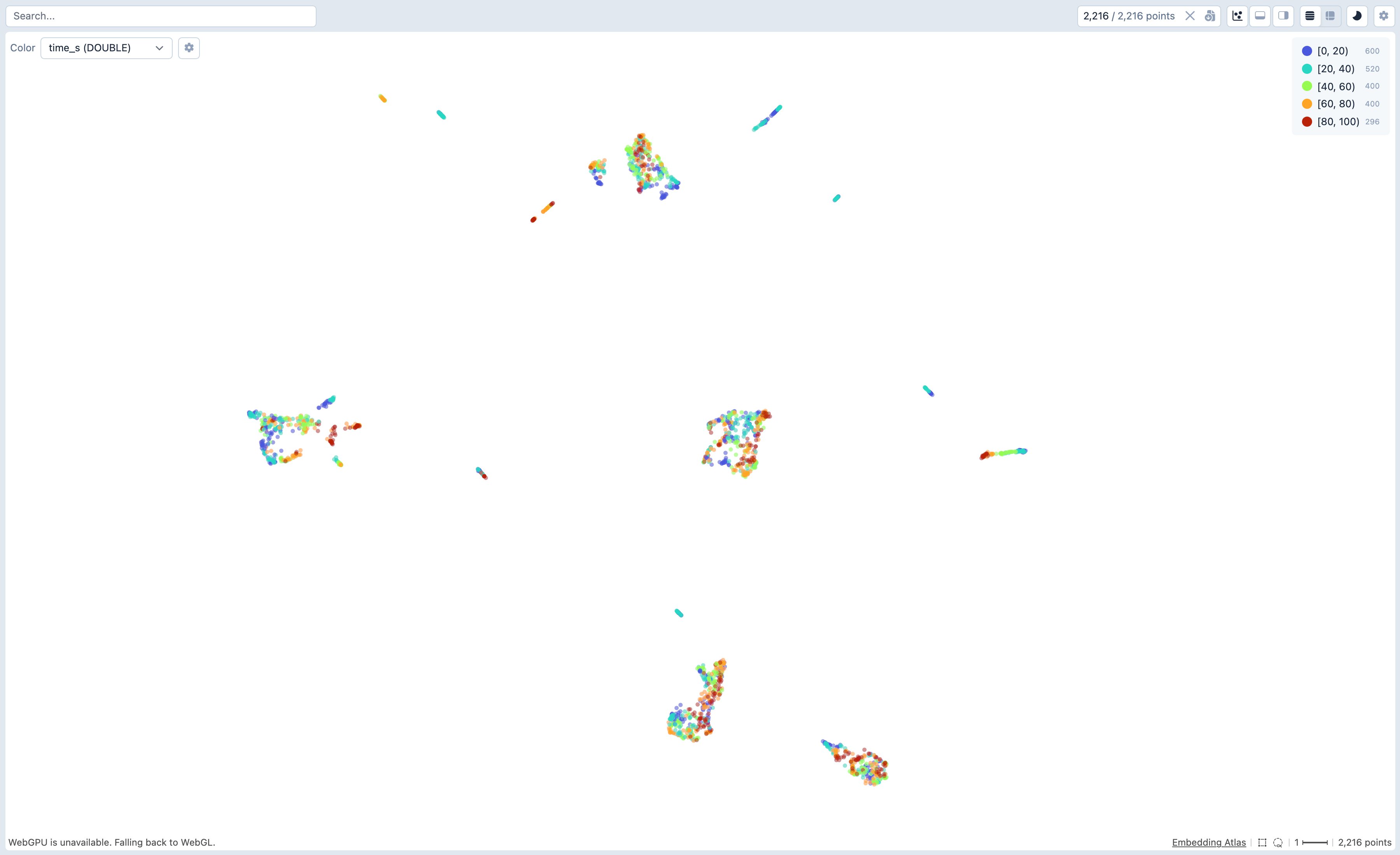Each tight cluster is one recording; the time gradient inside each cluster shows the trajectory of brain state during that recording.

## Try it yourself

Reproduce the figure above on a public EEG dataset:

```python theme={null}
import mne, torch, neuroencoder as ne
from neuroencoder import MRL
from mne.datasets import eegbci
mne.set_log_level("ERROR")

model = MRL.from_pretrained()

all_emb, all_files = [], []
for s in [1, 2, 3, 4, 5]:
    for r in [1, 2, 4, 6, 8, 10]:
        f = eegbci.load_data(subjects=s, runs=r, verbose=False)[0]
        raw = mne.io.read_raw_edf(f, preload=True, verbose=False)
        eegbci.standardize(raw)
        # Sliding window: 30s epochs, 1s hop
        images = ne.preprocess(
            raw.get_data(),
            sfreq=raw.info["sfreq"],
            channel_names=raw.ch_names,
            stride_seconds=1.0,
        )
        emb = model.predict(images, dim=192)
        all_emb.append(emb)
        all_files.extend([f.split("/")[-1]] * len(emb))

ne.explore(torch.cat(all_emb), filename=all_files, epoch_seconds=1.0)
```

## Defaults

|                   |                 |
| ----------------- | --------------- |
| Coloring          | time (auto-set) |
| Side charts panel | hidden          |
| Bottom data table | hidden          |
| Theme             | light           |
| Projection        | UMAP            |

Pass `show_charts=True` and / or `show_table=True` to re-enable the panels.

## Standalone server (no Jupyter)

```python theme={null}
ne.serve(embeddings, filename=filenames, port=5055)
```

Launches a localhost web app with the same defaults as `ne.explore()` — light theme, panels hidden, time coloring already applied. Opens in your default browser. Blocks until Ctrl-C.

## With filenames

Tag points with their source recording:

```python theme={null}
ne.explore(embeddings, filename=["recording_A.edf"] * 50 + ["recording_B.edf"] * 50)
```

## Sliding-window vs non-overlapping

For dense temporal visualizations, pass `stride_seconds` to `ne.preprocess`. Smaller strides give many more points per recording, revealing smooth trajectories.

```python theme={null}
# Default - non-overlapping 30s epochs
ne.preprocess(data, sfreq=256, channel_names=ch_names)

# Sliding 30s windows hopping every 1 second
ne.preprocess(data, sfreq=256, channel_names=ch_names, stride_seconds=1.0)
```

## Projection methods

```python theme={null}
ne.explore(embeddings, method="umap")    # default
ne.explore(embeddings, method="tsne")
ne.explore(embeddings, method="pca")
```

## Standalone server

For very large datasets, save to parquet and serve via the `embedding-atlas` CLI:

```bash theme={null}
embedding-atlas embeddings.parquet --x x --y y --neighbors neighbors
```

## Static plot

```python theme={null}
ne.plot(embeddings)                  # by time (default, viridis)
ne.plot(embeddings, color="cluster") # DBSCAN auto-clustering
ne.plot(embeddings, color=labels)    # custom values
```